Introduction
In Service Provider networking, there are little-known network devices known as Multiplexers. I say little-known because it isn’t taught in most networking courses. In this two part article we’ll explore a brief history of the multiplexer, how it works, and why it is the backbone of provider networking.
Why Are Multiplexers Needed
Multiplexers allow carriers to maximize the bandwidth of their physical cable infrastructure. The job of a multiplexer is to combine many signals from different inputs onto a single shared output for transport to another location. Multiplexers originated in the Bell System telephone network but these days they primarily transport Ethernet services. Multiplexers work by manipulating electrical and optical signals directly. This makes them layer 1 devices, though modern multiplexers can also operate at higher layers.
In my article A History of the Leased Line, I talk about different ways providers offer private circuits. Private circuits were one driving force behind the development of multiplexers. The other main force was carrier transport.
Carriers need to transport consumer data efficiently through their network as well. Historically this meant moving calls between local exchange telephone switches and between tandem switches that serviced entire area codes.
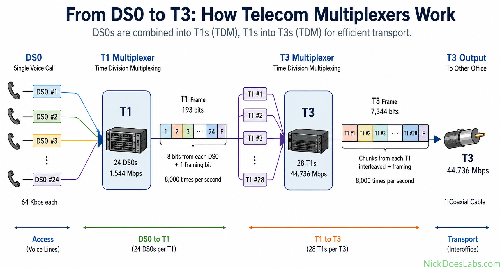
Multiplexing calls into T1s allowed carriers to transport 24 calls on a single T1. A T1 requires 4 wires, so this means using 44 less wires than transporting the calls individually. You can already see the benefit to multiplexing. A T3 can carry 28 T1s, that’s 672 calls on 1 coaxial cable. Clearly this is better than running 672 copper pairs between each local exchange.
So the benefit of multiplexing is now obvious, but how did it work in the old old days? Let’s go back to the beginning.
Early Multiplexers (Frequency Division Multiplexing)
Bell labs developed the first multiplexing technology in the early 1900s. This technology was known as frequency division multiplexing. Frequency division multiplexing worked by assigning different voice calls to different frequency channels. The combined signal of multiple channels could then be carried over one wire.
To do this, an analog voice signal passed through a circuit called a modulator which would replicate each waveform onto its assigned frequency. At the far end a demodulator would separate the frequencies back into individual waveforms on separate wires.
The equipment that did this was the 12-channel group. The 12 channel group gave each of the 12 calls their own 4 kHz frequency band, starting at 60kHz and ending at 108. This invention was followed by:
- Super Groups – 5 groups / 60 channels total
- Master Groups- 10 supergroups / 600 channels total
- Jumbo Groups- 6 Master groups / 3600 channels
Bell engineers figured out that Coaxial cable could carry much higher frequencies than twisted pair. This allowed them to put more and more channels on a single coaxial cable. This system became known as the L-Carrier system. The last L-Carrier standard was the L-5e released in 1975 which could carry 13,200 voice channels.
An interesting parallel to make note of here is that the L-Carrier system used essentially the same techniques that Cable TV still uses to this day (except for fiber).
The T-Carrier System
In the late 1950s and 1960s, the digital revolution was beginning. Bell Systems, always on the cutting edge, wanted a digital alternative to the L-Carrier. Going digital meant less analog distortion, smaller equipment, and better compatibility with computers. The solution they came up with was the T-Carrier system.
The basis of a digital signal is that it is composed of binary values, 1s or 0s. This is different from an analog signal where the waveform of the signal itself corresponds to a sound wave. An analog signal just needs to be amplified to produce audible sound. A digital voice signal must be sampled from an analog sound wave.
How are DS0s Sampled
In the T-Carrier system a DS0 represents a single voice call and is the building block of the T1. A DS0 is sampled by looking at the amplitude of the sound wave at a particular point in time. That amplitude is mapped to the nearest discrete “level”. This level is represented by 8 bits, aka one byte.
DS0s are sampled at a rate of 8khz or 8,000 times per second. This captures enough of the analog sound wave that it can be accurately reconstructed at the remote end. There is some loss of data in sampling but the human brain can’t detect it.
How T1s Multiplex DS0s (TDM)
A T1 takes 24 DS0 channels and assigns each DS0 to a time slot. This time slot is when that DS0s 8bits will be placed onto the wire. Each DS0 will get 8,000 of these 8bit time slots per second. This matches the sapling rate of the DS0 so there is no data loss when combining DS0s into a T1.
8,000 times per second the T1 will transmit 8 bits from each channel and one frame bit. This is known as Time division multiplexing (TDM) since channels were kept separate by dividing time into distinct slots. Synchronized timing was critical for multiplexers to keep channels in sync. The most popular DS0 to T1 Multiplexer was probably the D4 bank. The D4 bank was built by Western Electric and became widespread in the early 1980s.
How T3s Multiplex T1s & What is a T2?
A T1 carries 1.544 Mbps of data. A T3 combines 28 T1s into a single signal at 44.736 Mbps (with framing and overhead). A T3 can be thought of like a larger pipe being fed by 28 small garden hoses. The T3 accomplishes this by taking chunks of each T1s bit stream and interleaving them. Like the T1 this is done by giving each channel its own time slot.
There is something called a T2 or DS2 inside of T3 multiplexers. The T2 as a signal doesn’t leave the multiplexer at all, but it’s used inside the multiplexer for organization. A T2 holds 4 T1s, and 7 T2s make up a T3. T3 multiplexers like the Alcatel Lucent DDM-1000 actually had T2 line cards which would perform the T1 to T2 conversion.
How it all Connects
In the Central Office, DS0s would have interfaces on the Main Distribution Frame (MDF). Here, central office technicians would run twisted pair jumpers to cross-connect outside plant wire pairs to the D4 banks.
T1s would have interfaces on DSX panels. Technicians would run twisted pair cable to cross-connect DSX ports. This allowed them to connect the T1s from a D4 bank multiplexer to a T3 multiplexer for interoffice transport. PSTN switches like the DMS 100 and other equipment would also have DSX ports to receive and transmit T1s.
T3s would be cross-connected at a DSX3 panel. The DSX3 was similar to a DSX panel but it used coaxial cable instead of twisted pair.